wps表格日期计算天数

If you want to count the number of days between two dates, you can use the DAYS, DATEDIF, and NETWORKDAYS functions in Google Sheets to do so. DAYS and DATEDIF count all days, while NETWORKDAYS excludes Saturday and Sunday.

如果要计算两个日期之间的天数，可以使用Google表格中的DAYS，DATEDIF和NETWORKDAYS函数来进行计算。 DAYS和DATEDIF整天都在计数，而NETWORKDAYS不包括星期六和星期日。

计算两个日期之间的所有天数 (Counting All Days Between Two Dates)

To count the days between two dates, regardless of whether the day is a weekday or a holiday, you can use the DAYS or DATEDIF functions.

要计算两个日期之间的天数，无论一天是工作日还是假期，都可以使用DAYS或DATEDIF函数。

使用DAYS功能 (Using the DAYS Function)

The DAYS function is the easiest to use, so long as you’re not fussed about excluding holidays or weekend days. DAYS will take note of additional days held in a leap year, however.

DAYS函数是最易于使用的，只要您不必为假期或周末排除烦恼。 但是，DAYS将记录note年的其他日子。

To use DAYS to count between two days, open your  spreadsheet and click on an empty cell. Type =DAYS("01/01/2019","01/01/2018"), replacing the dates shown with your own.

要使用DAYS进行两天之间的计数，请打开电子表格，然后单击一个空白单元格。 输入=DAYS("01/01/2019","01/01/2018") ，将显示的日期替换为您自己的日期。

Use your dates in reverse order, so put the end date first, and the start date second. Using the start date first will result in DAYS returning a negative value.

按相反的顺序使用日期，因此将结束日期放在第一位，将开始日期放在第二位。 首先使用开始日期将导致DAYS返回负值。

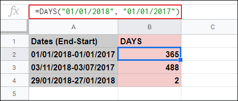
As the example above shows, the DAYS function counts the total number of days between two specific dates. The date format used in the example above is the U.K. format, DD/MM/YYYY. If you’re in the U.S., make sure you use MM/DD/YYYY.

如上面的示例所示，DAYS函数计算两个特定日期之间的总天数。 上例中使用的日期格式是英国格式DD / MM / YYYY。 如果您在美国，请确保使用MM / DD / YYYY。

You’ll need to use the default date format for your locale. If you want to use a different format, click File > Spreadsheet Settings and change the “Locale” value to another location.

您需要为您的语言环境使用默认的日期格式。 如果要使用其他格式，请单击文件>电子表格设置，然后将“区域设置”值更改为另一个位置。

You can also use the DAYS function with cell references. If you’ve specified two dates in separate cells, you can type =DAYS(A1, A11), replacing the A1 and A11 cell references with your own.

您还可以将DAYS函数与单元格引用一起使用。 如果您在单独的单元格中指定了两个日期，则可以键入=DAYS(A1, A11) ，用自己的A1和A11单元格引用替换。

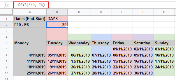
In the example above, a difference of 29 days is recorded from dates held in cells E6 and F10.

在上面的示例中，与保存在单元格E6和F10中的日期相比，相差29天。

使用DATEDIF函数 (Using the DATEDIF Function)

An alternative to DAYS is the DATEDIF function, which allows you to calculate the number of days, months, or years between two set dates.

DAYS的替代方法是DATEDIF函数，它使您可以计算两个设置日期之间的天数，月数或年数。

Like DAYS, DATEDIF takes leap days into account and will calculate all days, rather than limit you to business days. Unlike DAYS, DATEDIF doesn’t work in reverse order, so use the start date first and the end date second.

与DAYS一样，DATEDIF也将leap日纳入考虑范围，并将计算整天，而不是将您限制在工作日内。 与DAYS不同，DATEDIF不能以相反的顺序工作，因此请首先使用开始日期，然后使用结束日期。

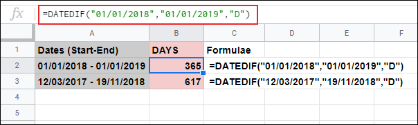
If you want to specify the dates in your DATEDIF formula, click on an empty cell and type =DATEDIF("01/01/2018","01/01/2019","D"), replacing the dates with your own.

如果要在DATEDIF公式中指定日期，请单击一个空单元格，然后键入=DATEDIF("01/01/2018","01/01/2019","D") ，然后用您自己的日期替换。

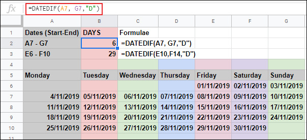
If you want to use dates from cell references in your DATEDIF formula, type =DATEDIF(A7,G7,"D"), replacing the A7 and G7 cell references with your own.

如果要在DATEDIF公式中使用单元格引用中的日期，请键入=DATEDIF(A7,G7,"D") ，将A7和G7单元格引用替换为您自己的引用。

计算两个日期之间的工作日 (Counting Business Days Between Two Dates)

The DAYS and DATEDIF functions allow you to find the days between two dates, but they count all days. If you want to count business days only, and you want to discount additional holiday days, you can use the NETWORKDAYS function.

DAYS和DATEDIF函数使您可以查找两个日期之间的日期，但它们是一整天。 如果您只想计算工作日，并且想打折额外的假期，则可以使用NETWORKDAYS函数。

NETWORKDAYS treats Saturday and Sunday as weekend days, discounting these during its calculation. Like DATEDIF, NETWORKDAYS uses the start date first, followed by the end date.

NETWORKDAYS将周六和周日视为周末，并在计算时将其打折。 与DATEDIF一样，NETWORKDAYS首先使用开始日期，然后使用结束日期。

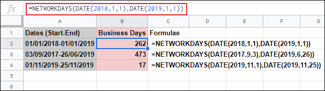
To use NETWORKDAYS, click on an empty cell and type =NETWORKDAYS(DATE(2018,01,01),DATE(2019,01,01)). Using a nested DATE function allows you to convert years, months, and dates figures into a serial date number, in that order.

要使用NETWORKDAYS，请单击一个空单元格并键入=NETWORKDAYS(DATE(2018,01,01),DATE(2019,01,01)) 。 使用嵌套的DATE函数，可以按此顺序将年，月和日期数字转换为序列日期数字。

Replace the figures shown with your own year, month, and date figures.

将显示的数字替换为您自己的年，月和日期数字。

You can also use cell references within your NETWORKDAYS formula, instead of a nested DATE function.

您还可以在NETWORKDAYS公式中使用单元格引用，而不是嵌套的DATE函数。

Type =NETWORKDAYS(A6,B6) in an empty cell, replacing the A6 and B6 cell references with your own.

在一个空单元格中键入=NETWORKDAYS(A6,B6) ，用您自己的A6和B6单元格引用替换。

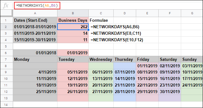
In the above example, the NETWORKDAYS function is used to calculate the working business days between various dates.

在上面的示例中，NETWORKDAYS函数用于计算各个日期之间的工作日。

If you want to exclude certain days from your calculations, like days of certain holidays, you can add these at the end of your NETWORKDAYS formula.

如果要从计算中排除某些天，例如某些假期的天，则可以在NETWORKDAYS公式的末尾添加这些天。

To do that, click on an empty cell and type =NETWORKDAYS(A6,B6,{B6:D6}. In this example, A6 is the start date, B6 is the end date, and the B6:D6 range is a range of cells containing days of holidays to be excluded.

为此，请单击一个空单元格，然后键入=NETWORKDAYS(A6,B6,{B6:D6} 。在此示例中，A6是开始日期，B6是结束日期，B6：D6范围是一个范围包含假期天数的单元格将被排除。

You can replace the cell references with your own dates, using a nested DATE function, if you’d prefer. To do this, type =NETWORKDAYS(E11,F13,{DATE(2019,11,18),DATE(2019,11,19)}), replacing the cell references and DATE criteria with your own figures.

如果愿意，可以使用嵌套的DATE函数用自己的日期替换单元格引用。 为此，请键入=NETWORKDAYS(E11,F13,{DATE(2019,11,18),DATE(2019,11,19)}) ，用您自己的数字替换单元格引用和DATE条件。

In the above example, the same range of dates is used for three NETWORKDAYS formulae. With 11 standard business days reported in cell B2, between two and three additional holiday days are removed in cells B3 and B4.

在上面的示例中，三个NETWORKDAYS公式使用相同的日期范围。 由于在单元格B2中报告了11个标准工作日，因此在单元格B3和B4中又删除了两到三个假日。

翻译自:

wps表格日期计算天数